LSTM Time Series Knowledge
briefly talk about LSTM time series with example
LSTM
LSTM is a variant of RNN used in deep learning, and can be used LSTMs when working on sequences of data.
- Time series forecasting (for example, stock prediction)
- Text generation
- Video classification
- Music Generation
- Anomaly detection
RNNs are neural networks that are good with sequential data. It can be video, audio, text, stock market time series, or even a single image cut into a sequence of its parts.
Compare: Standard neural networks (convolutional or vanilla) have one major shortcoming when compared to RNNs - they cannot reason about previous inputs to inform later ones.
LSTM vs RNN
- Typical RNNs can’t memorize long sequences. The effect called “vanishing gradients” happens during the backpropagation phase of the RNN cell network. The gradients of cells that carry information from the start of a sequence go through matrix multiplications by small numbers and reach close to 0 in long sequences. In other words - information at the start of the sequence has almost no effect at the end of the sequence.
- LSTM is an RNN architecture that can memorize long sequences - up to 100s of elements in a sequence. LSTM has a memory gating mechanism that allows the long-term memory to continue flowing into the LSTM cells.
Core idea
- The LSTM does have the ability to remove or add information to the cell state, carefully regulated by structures called gates.
Memory Gate
- Information in LSTMs can be stored, written, or read via gates that open and close. These gates store the memory in the analog format, implementing element-wise multiplication by sigmoid ranges between 0-1. Analog, being differentiable in nature, is suitable for backpropagation.
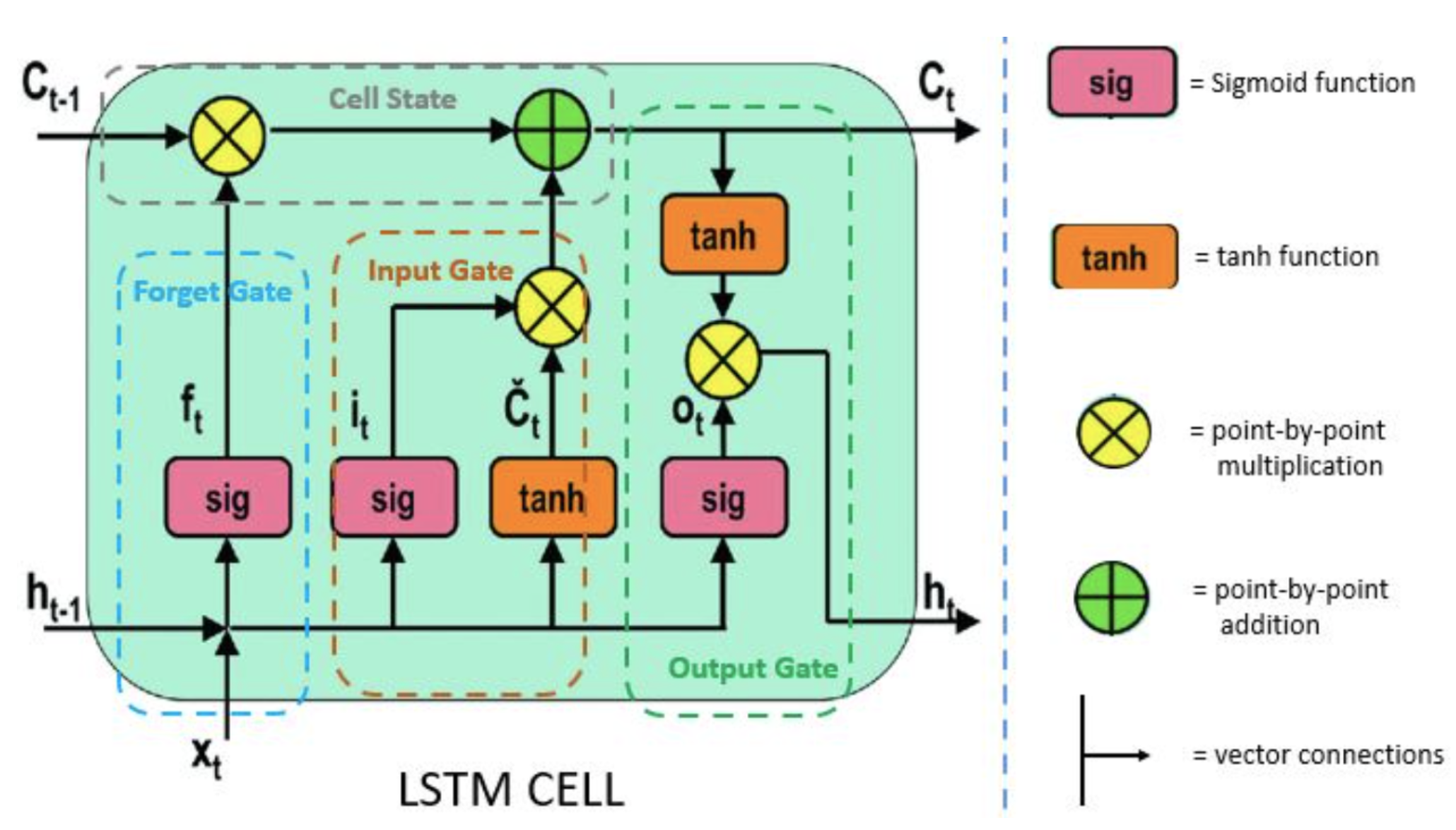
- Architecture of LSTM:
- Tanh: Non-linear activation function. It regulates the values flowing through the network, maintaining the values between -1 and 1.</li>
- Sigmoid: Non-linear activation functions. It is contained by the gate, values between 0 and 1. It helps the network to update or forget the data. multiplication = 0 -> forgotten; = 1 -> information stays.
- Forget gate: input: current and hidden; output: f(t) values between 0 and 1
- Decide which information needs attention and which can be ignored.
- The information from the current input X(t) and hidden state h(t-1) are passed through the sigmoid function.
Sigmoid generates values between 0 and 1. It concludes whether the part of the old output is necessary (by giving the output closer to 1). This value of f(t) will later be used by the cell for point-by-point multiplication.
- Input gate: input: current state X(t) and previously hidden state h(t-1); output: vector (C~(t)) with all the possible values between -1 and 1
- Update the cell status.
- First, the current state X(t) and previously hidden state h(t-1) are passed into the second sigmoid function. The values are transformed between 0 (important) and 1 (not important). Next, the same information of the hidden state and current state will be passed through the tanh function which will create a vector (C~(t)) with all the possible values between -1 and 1. The output values generated from the activation functions are ready for point-by-point multiplication.
- Cell state operation: input: new state after forget and input; output: updates the cell state to C(t)
- Decide and store the information from the new state in the cell state, after having information from the forget and input gate.
- The previous cell state C(t-1) gets multiplied with forget vector f(t). If the outcome is 0, then values will get dropped in the cell state.
- Next, the network takes the output value of the input vector i(t) and performs point-by-point addition, which updates the cell state giving the network a new cell state C(t).
- Output gate: input: values of the current state and previous hidden state; output: new cell state and new hidden state
- Determines the value of the next hidden state. This state contains information on previous inputs.
- First, the values of the current state and previous hidden state are passed into the third sigmoid function. Then the new cell state generated from the cell state is passed through the tanh function. Both these outputs are multiplied point-by-point. Based on the final value, the network decides which information the hidden state should carry. This hidden state is used for prediction.
- Finally, the new cell state and new hidden state are carried over to the next time step.
- Overall, forget gate determines which relevant information from the prior steps is needed. The input gate decides what relevant information can be added from the current step, and the output gate finalizes the next hidden state.

Hyperparameters to tune
- Number of nodes and hidden layers.
- Number of units in dease layer: A dense layer is the most frequently used layer which is basically a layer where each neuron receives input from all neurons in the previous layer.
- Dropout: Helps avoid overfitting in training by bypassing randomly selected neurons, thereby reducing the sensitivity to specific weights of the individual neurons.
- Activation functions.
- Learning rate: Setting a higher learning rate accelerates the learning but the model may not converge. Conversely, a lower rate will slow down the learning drastically as steps towards the minimum of loss function will be tiny but will allow the model to converge smoothly.
- Batch size: Large sizes make large gradient steps compared to smaller ones for the same number of samples “seen”.
LSTM RNN Beer Wine and Distilled Alcoholic Beverages Sales
An example project (please use Google Colab Notebook) employed LSTM time series RNN to forecast wine prices, leveraging the temporal patterns in historical wine pricing data